Tutorial: Satellite Sensor & Software Malfunctions

This tutorial demonstrates realistic satellite malfunction effects through hands-on examples. Each tutorial recreates documented remote sensing failures, from early mission degradation to the famous Landsat 7 SLC-Off failure and extreme glitch art aesthetics.

Prerequisites

• sevenrad-stills installed and configured (Installation Guide)
• Basic familiarity with YAML pipeline system (YAML Pipeline System)

Tutorial Overview

Tutorial	Operations Used	Simulates	Difficulty
01-Landsat 7 SLC-Off	slc_off	May 31, 2003 Scan Line Corrector failure	Beginner
02-Early Mission	salt_pepper, corduroy	Years 1-3 baseline degradation	Beginner
03-Late Mission	salt_pepper, corduroy, buffer_corruption, compression_artifact	Years 15+ accumulated failures	Intermediate
04-Glitch Art	All 6 operations	Extreme artistic aesthetics	Advanced

Common Video Source

All tutorials use the same video segment:

source:
  youtube_url: "https://www.youtube.com/watch?v=MzJaP-7N9I0"

segment:
  start: 192.0    # 3 minutes 12 seconds (3m12s)
  end: 195.0      # 3 minutes 15 seconds (3m15s)
  interval: 0.0667  # 15 frames per second = 45 total frames

Why these settings?

• 3 seconds: Sufficient variety to show effects
• 15 fps: Good temporal resolution
• 45 frames: Enough to see frame-to-frame patterns
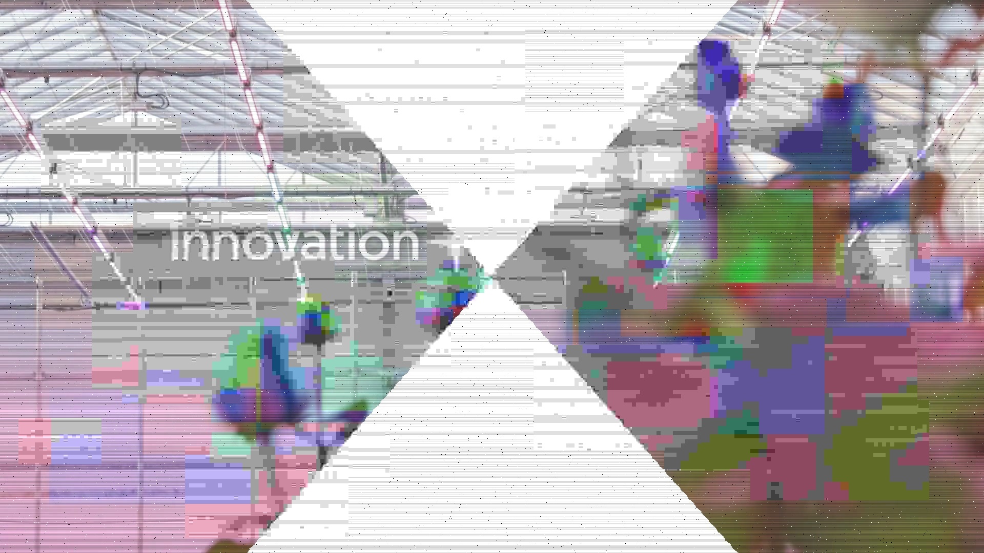
• Video content: Growing roses scene provides diverse colors and textures

Original Frame (frame 15, before any operations):

---

Tutorial 1: Landsat 7 SLC-Off Simulation

Goal: Accurately recreate the iconic Landsat 7 Enhanced Thematic Mapper Plus (ETM+) Scan Line Corrector failure that occurred on May 31, 2003.

Real-world context: This famous mechanical failure affected all Landsat 7 data from 2003 onwards, creating characteristic diagonal wedge-shaped gaps in a zig-zag pattern, widening from center to edges (~22% data loss at scene edges).

Running the Tutorial

The tutorial YAML is located at:

docs/tutorials/satellite-malfunctions/01-landsat7-slcoff.yaml

Run:

sevenrad pipeline docs/tutorials/satellite-malfunctions/01-landsat7-slcoff.yaml

Expected Results

Output: tutorials/satellite-malfunctions/01-landsat7-slcoff/final/ (45 frames)

Visual Characteristics:

• Diagonal wedge-shaped gaps in zig-zag pattern
• Gaps alternate direction (left/right) on each scan line
• No gaps at center (nadir point), maximum at top/bottom edges
• Black-filled gaps showing missing data
• Diagonal offset simulating uncompensated forward satellite motion

Parameter Explanation

gap_width: 0.22    # Historical 22% maximum gap at edges
scan_period: 14    # Scan line spacing (ETM+ geometry)
fill_mode: "black" # Show missing data as black

• gap_width: 0.22 - Matches historical Landsat 7 maximum gap (22% of scene width)
• scan_period: 14 - Approximates ETM+ scan line spacing
• fill_mode: "black" - Visualizes missing data regions

Historical Accuracy

This simulation matches the real Landsat 7 SLC-Off geometry:

1. Scan Line Corrector mirror mechanism failed
2. Forward spacecraft motion no longer compensated
3. Creates diagonal gaps with alternating directions (zig-zag)
4. Gap width proportional to distance from nadir (center)
5. Diagonal offset of 0.3 pixels/row creates shallow angle
6. Gaps span multiple rows matching scan_period duration

Timeline:

• May 31, 2003: SLC failure occurred
• 2003-2024: 21+ years of operation with this artifact
• Impact: 14% average data loss, 22% maximum at edges

What You’ll Learn

• How mechanical failures create geometric artifacts
• Understanding diagonal wedge-shaped gap patterns
• Historical satellite mission failures
• Scientific accuracy in simulation parameters

---

Tutorial 2: Early Mission Degradation

Goal: Simulate a satellite in years 1-3 of operation with minimal degradation - baseline cosmic ray hits and slight calibration drift.

Real-world context: New satellites in Low Earth Orbit experience baseline cosmic ray flux and minor detector calibration variations from manufacturing differences.

Running the Tutorial

The tutorial YAML is located at:

docs/tutorials/satellite-malfunctions/02-early-mission.yaml

Run:

sevenrad pipeline docs/tutorials/satellite-malfunctions/02-early-mission.yaml

Expected Results

Output:

• Final: tutorials/satellite-malfunctions/02-early-mission/final/ (45 frames)
• Intermediate: tutorials/satellite-malfunctions/02-early-mission/intermediate/ (step-by-step)

Visual Characteristics:

• Very sparse random white/black pixels (cosmic rays)
• Subtle vertical lines barely visible (calibration drift)
• Overall high image quality typical of new satellite

Progressive Steps:

Step 1: Cosmic Ray Hits Only

Sparse white/black pixels from cosmic ray impacts on detector (0.01% of pixels affected).

Step 2: Final Result (Cosmic Rays + Detector Drift)

Subtle vertical striping added from detector calibration variations (30% of columns with ±2% brightness variation).

Parameter Explanation

# Step 1: Cosmic ray hits
salt_pepper:
  amount: 0.0001         # 0.01% of pixels (baseline LEO rate)
  salt_vs_pepper: 0.5    # Equal white/black probability
  seed: 42

# Step 2: Detector calibration drift
corduroy:
  strength: 0.1          # Subtle ±2% brightness variation
  orientation: "vertical" # Push-broom scanner
  density: 0.3           # 30% of detector elements
  seed: 100

Scientific Context

Early mission parameters based on:

• Landsat 8/9 OLI performance (years 0-3)
• Terra/Aqua MODIS baseline noise
• Sentinel-2 MSI early mission data quality

Orbital Environment:

• Low Earth Orbit (600-800 km altitude)
• Moderate cosmic ray flux
• Minimal radiation damage accumulation
• Calibration coefficients still accurate

What You’ll Learn

• Baseline satellite image quality
• Combining sensor-level effects
• Realistic early-mission parameters
• Using seeds for reproducibility

---

Tutorial 3: Late Mission Degradation

Goal: Simulate a satellite in years 15+ of operation with accumulated radiation damage, calibration drift, and occasional transmission errors.

Real-world context: Long-duration missions accumulate significant degradation: detector damage, severe calibration drift, memory upsets, and encoder stress.

Running the Tutorial

The tutorial YAML is located at:

docs/tutorials/satellite-malfunctions/03-late-mission.yaml

Run:

sevenrad pipeline docs/tutorials/satellite-malfunctions/03-late-mission.yaml

Expected Results

Output:

• Final: tutorials/satellite-malfunctions/03-late-mission/final/ (45 frames)
• Intermediate: Shows progressive degradation through 4 steps

Visual Characteristics:

• Dense random white pixels (hot pixels from radiation)
• Strong vertical banding across entire image
• Rectangular “glitch blocks” with bitwise corruption
• Blocky JPEG artifacts (8x8 DCT blocks) in random regions
• Combined realistic aging satellite appearance

Progressive Steps:

Step 1: Radiation Damage (Salt & Pepper)

Dense white/black pixels from 15+ years of accumulated cosmic ray damage (0.2% of pixels affected, biased toward “salt” hot pixels).

Step 2: + Calibration Drift (Corduroy)

Strong vertical banding added from severe detector calibration drift (60% of columns with ±14% brightness variation).

Step 3: + Memory Corruption (Buffer Corruption)

Rectangular “glitch blocks” with XOR bitwise corruption from cosmic ray hits on memory chips (3 corrupted tiles).

Step 4: Final Result (+ Encoder Stress)

Severe JPEG compression artifacts added from aging on-board encoder hardware (5 tiles at quality 8).

Operations Applied

1. radiation_damage (salt_pepper)     # 0.2% pixels affected
2. calibration_drift (corduroy)       # ±14% brightness variation
3. memory_upsets (buffer_corruption)  # 3 corrupted blocks (XOR)
4. encoder_stress (compression_artifact) # 5 tiles at quality 8

Aging Mechanisms

• Radiation damage: 15+ years of cosmic ray hits create permanent hot pixels
• Calibration drift: Thermal cycling and radiation exposure
• Memory upsets: Normal cosmic ray SEU rate in buffers
• Encoder stress: Hardware aging and thermal issues

Scientific Context

Late mission parameters based on:

• Landsat 5 final years (28+ years operational)
• Terra MODIS degradation (20+ years)
• NOAA AVHRR long-duration missions

What You’ll Learn

• How failures compound over time
• Multiple simultaneous malfunction types
• Realistic operation ordering
• Creating complex degradation aesthetics

---

Tutorial 4: Satellite Glitch Art

Goal: Create extreme digital aesthetics using exaggerated satellite malfunction parameters for artistic expression and visual experimentation.

Real-world context: While not scientifically realistic, this tutorial uses all 6 satellite operations with extreme parameters to create intentional glitch art aesthetics.

Running the Tutorial

The tutorial YAML is located at:

docs/tutorials/satellite-malfunctions/04-glitch-art.yaml

Run:

sevenrad pipeline docs/tutorials/satellite-malfunctions/04-glitch-art.yaml

Performance Note: This pipeline is computationally expensive (20 JPEG encode/decode cycles per frame). Expected runtime: 2-5 minutes.

Expected Results

Output:

• Final: tutorials/satellite-malfunctions/04-glitch-art/final/ (45 frames)
• Intermediate: All 6 steps preserved showing progressive destruction

Visual Characteristics:

• Massive white diagonal gaps creating abstract geometry
• Wrong color channels in random blocks (BGR swaps)
• Shuffled RGB channels creating surreal colors
• Heavy horizontal banding across entire image
• Dense white/black pixel noise creating texture
• Severe 8x8 JPEG blocking in random regions
• Combined: Total digital destruction

Progressive Steps:

Step 1: Massive SLC-Off Gaps

Extreme 50% diagonal gaps with white fill creating dramatic geometric abstraction.

Step 3: + Band Swaps + Buffer Corruption

Color chaos from 15 BGR-swapped tiles plus 10 channel-shuffled blocks creating surreal palette.

Step 5: + Corduroy + Salt & Pepper

Heavy horizontal banding (±20%) and dense noise texture (0.5% pixels) creating digital static effect.

Step 6: Final Result (+ Compression Destruction)

Severe JPEG artifacts at quality 1 applied to 20 tiles, creating total digital destruction with 8x8 DCT blocking.

Operations Applied

1. massive_gaps (slc_off)              # 50% gaps, white fill
2. color_chaos (band_swap)             # 15 BGR-swapped tiles
3. buffer_mayhem (buffer_corruption)   # 10 channel-shuffled blocks
4. extreme_banding (corduroy)          # ±20% horizontal stripes
5. static_texture (salt_pepper)        # 0.5% dense noise
6. compression_destruction (compression_artifact) # 20 tiles, quality 1

Artistic Intent

This tutorial prioritizes visual impact over scientific accuracy:

• Abstract geometric patterns (SLC-Off gaps)
• Color field disruptions (band swaps, buffer corruption)
• Digital texture (salt & pepper, compression)
• Rhythmic visual patterns (corduroy banding)

Aesthetic References

• Glitch art (Rosa Menkman, Phillip Stearns)
• Data moshing aesthetics
• Databending and circuit bending
• Digital decay and corruption aesthetics
• Satellite imagery as abstract art

What You’ll Learn

• Combining all 6 satellite operations
• Exaggerating parameters for artistic effect
• Operation ordering for layered aesthetics
• Creating intentional digital destruction

---

Advanced Topics

Operation Ordering

Order matters when combining operations:

Realistic order (sensor → transmission → geometric):

steps:
  - operation: "salt_pepper"       # Sensor level
  - operation: "corduroy"          # Detector level
  - operation: "buffer_corruption" # Memory level
  - operation: "compression_artifact" # Encoding level
  - operation: "band_swap"         # Transmission level
  - operation: "slc_off"           # Geometric level

Artistic order (for specific aesthetics):

# SLC gaps THEN corruption (gaps have clean edges)
steps:
  - operation: "slc_off"
  - operation: "buffer_corruption"

# Corruption THEN SLC (corrupted data visible in gaps with mean fill)
steps:
  - operation: "buffer_corruption"
  - operation: "slc_off"
    params:
      fill_mode: "mean"  # Shows corrupted data in gaps

Seed Management

Consistent corruption across frames:

params:
  seed: 42  # Same pattern every frame

Frame-varying corruption:

# Don't specify seed - random each frame
params:
  tile_count: 5
  # No seed parameter

Parameter Tuning Guide

For subtle, realistic effects:

• salt_pepper amount: 0.0001 - 0.001
• corduroy strength: 0.1 - 0.3
• buffer_corruption severity: 0.2 - 0.4
• compression_artifact quality: 15 - 20
• slc_off gap_width: 0.05 - 0.15

For dramatic, artistic effects:

• salt_pepper amount: 0.005 - 0.02
• corduroy strength: 0.6 - 1.0
• buffer_corruption severity: 0.7 - 1.0
• compression_artifact quality: 1 - 5
• slc_off gap_width: 0.3 - 0.5

---

Troubleshooting

band_swap Fails on Grayscale Video

Problem: ValueError: Band swap requires RGB or RGBA image

Solution: Grayscale videos don’t have RGB channels to swap. Use buffer_corruption with xor or invert instead:

- operation: "buffer_corruption"
  params:
    corruption_type: "xor"  # Works on grayscale
    severity: 0.5

No Visible SLC Gaps

Problem: SLC gaps not appearing in output

Solutions:

1. Check gap_width - must be > 0.0
2. Verify scan_period isn’t larger than image height
3. Try fill_mode: "black" or "white" for more obvious gaps
4. Ensure diagonal pattern is visible (not just horizontal)

Operations Too Subtle

Problem: Can’t see malfunction effects

Solutions:

1. Increase severity/strength/amount parameters
2. Use lower quality values (compression_artifact: 1-5)
3. Increase tile_count or density
4. Check intermediate steps to see each operation in isolation

Color Corruption Not Happening

Problem: band_swap or buffer_corruption channel_shuffle has no effect

Solutions:

1. Ensure image is RGB/RGBA (not grayscale)
2. Increase tile_count for more coverage
3. For channel_shuffle, ensure severity > 0.5 for visible changes
4. Verify permutation parameter is specified (band_swap)

---

Next Steps

After completing these tutorials:

1. Experiment with parameters - Adjust amounts, strengths, and qualities
2. Create custom combinations - Mix operations in new ways
3. Study real satellite data - Compare to actual Landsat, MODIS, or Sentinel imagery
4. Apply to your projects - Use for glitch art, book illustrations, or research
5. Read comprehensive docs:
   • Satellite Operations Reference - Complete parameter specifications
   • Technical Background - Real satellite failure modes

Questions or Issues?

• Check Satellite Operations Reference for parameter details
• Read Technical Background for scientific context
• Report issues on the project repository

---

Happy experimenting with satellite malfunction simulations!